GitHub Newsletter Discord

Version: 0.6.1

Portfolio Allocation

In this quick tutorial, the portfolio allocation problem shall be investigated. Of course, this is not financial advice in any way but should illustrate how multi-objective optimization can be applied to a quite interesting problem.

Let us start by loading some data for illustration purposes. Feel free to use your own.

import pandas as pd
import numpy as np
from pymoo.util.remote import Remote

file = Remote.get_instance().load("examples", "portfolio_allocation.csv", to=None)
df = pd.read_csv(file, parse_dates=True, index_col="date")

This tutorial is based on the Markowitz Mean-Variance Portfolio Theory and thus, we need to calculate the mean returns and covariances:

Info

Note that the problem in this case study can be solved directly using a quadratic solver (which will be much more efficient). However, such a solver finds only a single solution and must run multiple times to approximate the Pareto-optimal front. Moreover, it is worth noting that if we slightly change the problem to cubic or non-polynomial, it can not be applied anymore. The method shown provides more flexibility, for instance, optimizing objectives derived from Monte-Carlo sampling.

returns = df.pct_change().dropna(how="all")
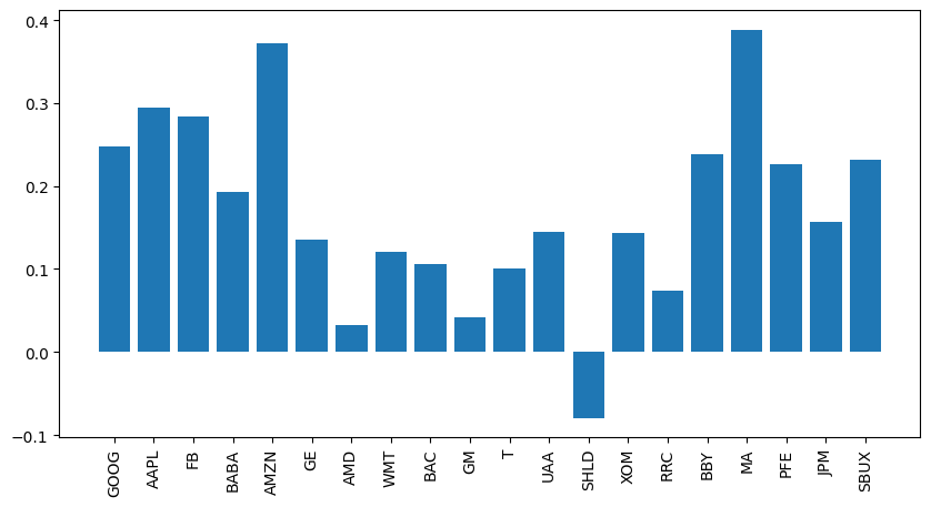
mu = (1 + returns).prod() ** (252 / returns.count()) - 1
cov = returns.cov() * 252

mu, cov = mu.to_numpy(), cov.to_numpy()

labels = df.columns

import matplotlib.pyplot as plt
fig, ax = plt.subplots(figsize=(10, 5))
k = np.arange(len(mu))
ax.bar(k, mu)
ax.set_xticks(k, labels, rotation = 90)
plt.show()


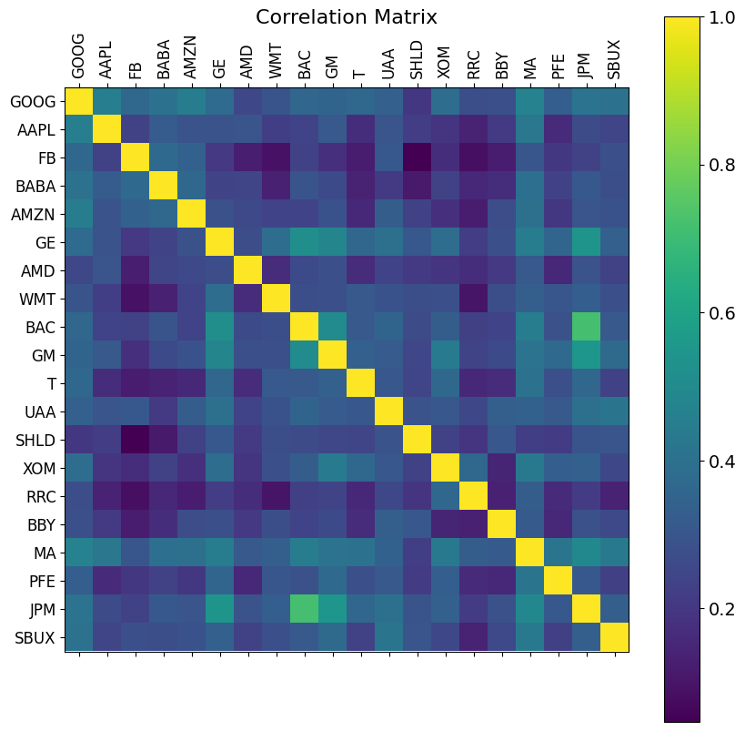
f = plt.figure(figsize=(10, 10))
plt.matshow(returns.corr(), fignum=f.number)
plt.xticks(k, labels, fontsize=12, rotation=90)
plt.yticks(k, labels, fontsize=12)
cb = plt.colorbar()
cb.ax.tick_params(labelsize=14)
plt.title('Correlation Matrix', fontsize=16)
print("DONE")

DONE

Then let us define an optimization problem based on the theory mentioned above:

from pymoo.core.problem import ElementwiseProblem

class PortfolioProblem(ElementwiseProblem):

    def __init__(self, mu, cov, risk_free_rate=0.02, **kwargs):
        super().__init__(n_var=len(df.columns), n_obj=2, xl=0.0, xu=1.0, **kwargs)
        self.mu = mu
        self.cov = cov
        self.risk_free_rate = risk_free_rate

    def _evaluate(self, x, out, *args, **kwargs):
        exp_return = x @ self.mu
        exp_risk = np.sqrt(x.T @ self.cov @ x)
        sharpe = (exp_return - self.risk_free_rate) / exp_risk

        out["F"] = [exp_risk, -exp_return]
        out["sharpe"] = sharpe

Now, we should consider one more fact. The variable x defines what percentage we will invest in what product. Thus, it can not be more than 100% in total. Moreover, an investment of a very small fraction does not really make sense. Thus we also incorporate each weight to be at least 1e-3 of the overall investment.

To ensure both, we can use a Repair operator (also see here) which will directly be used by the optimization method.

from pymoo.core.repair import Repair

class PortfolioRepair(Repair):

    def _do(self, problem, X, **kwargs):
        X[X < 1e-3] = 0
        return X / X.sum(axis=1, keepdims=True)

Now let us see what solutions are found to be optimal:

from pymoo.algorithms.moo.sms import SMSEMOA
from pymoo.optimize import minimize

problem = PortfolioProblem(mu, cov)

algorithm = SMSEMOA(repair=PortfolioRepair())

res = minimize(problem,
               algorithm,
               seed=1,
               verbose=False)

The algorithm has obtained a Pareto-optimal set trading off the mean return and volatility of the portfolio.

X, F, sharpe = res.opt.get("X", "F", "sharpe")
F = F * [1, -1]
max_sharpe = sharpe.argmax()

plt.scatter(F[:, 0], F[:, 1], facecolor="none", edgecolors="blue", alpha=0.5, label="Pareto-Optimal Portfolio")
plt.scatter(cov.diagonal() ** 0.5, mu, facecolor="none", edgecolors="black", s=30, label="Asset")
plt.scatter(F[max_sharpe, 0], F[max_sharpe, 1], marker="x", s=100, color="red", label="Max Sharpe Portfolio")
plt.legend()
plt.xlabel("expected volatility")
plt.ylabel("expected return")
plt.show()

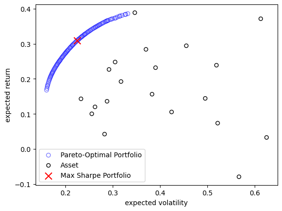
A common way for the decision making is looking at the sharpe ratio shown below:

import operator

allocation = {name: w for name, w in zip(df.columns, X[max_sharpe])}
allocation = sorted(allocation.items(), key=operator.itemgetter(1), reverse=True)

print("Allocation With Best Sharpe")
for name, w in allocation:
    print(f"{name:<5} {w}")

Allocation With Best Sharpe
MA    0.364421440541109
FB    0.20874148720289187
PFE   0.19574628824693652
AAPL  0.0769256140818164
BABA  0.07129945833640815
AMZN  0.04478765737146619
GOOG  0.03068450348113022
BBY   0.00739355073824167
GE    0.0
AMD   0.0
WMT   0.0
BAC   0.0
GM    0.0
T     0.0
UAA   0.0
SHLD  0.0
XOM   0.0
RRC   0.0
JPM   0.0
SBUX  0.0

<< Subset Selection Problem

Performance Indicator >>