GitHub Newsletter Discord

Version: 0.6.1

Convergence

It is fundamentally important to keep track of the convergence of an algorithm. Convergence graphs visualize the improvement over time, which is vital to evaluate how good the algorithm performance or what algorithms perform better. In pymoo different ways of tracking the performance exists. One is to store the whole algorithms run using the save_history flag and extract the necessary information for post-processing. Since history includes a deep copy, this can become memory intensive if many iterations are run. An alternative is to use a Callback object to just store the information needed and use them later on for plotting. Both ways are explained in the following for an unconstrained single-objective problem. Please bear in mind if your optimization problem has constraints or more than one objective, this needs to be addressed in the convergence curve (for instance, via plotting the CV, too, or using multi-objective optimization performance metrics).

History

Run your algorithm on the corresponding problem and make sure the save_history flag is enabled when calling the minimize function.

from pymoo.algorithms.soo.nonconvex.pso import PSO
from pymoo.problems import get_problem
from pymoo.optimize import minimize

problem = get_problem("ackley")
algorithm = PSO()

res = minimize(problem,
               algorithm,
               termination=('n_gen', 50),
               seed=1,
               save_history=True)

This creates a deep copy of the algorithm in each generation.

len(res.history)

50

This might be even more data than necessary and, therefore, not always the most memory-efficient method to use. However, if the number of generations is only a few hundred and the problem and algorithm objects do not contain a large amount of data, this shall be not a big deal. Using the history, we can extract the number of function evaluations and the optimum stored in the algorithm object at each generation/iteration. The algorithm object has the attribute opt (a Population object), which contains the current optimum. For single-objective algorithms, this is known to be only a single solution.

import numpy as np
import matplotlib.pyplot as plt

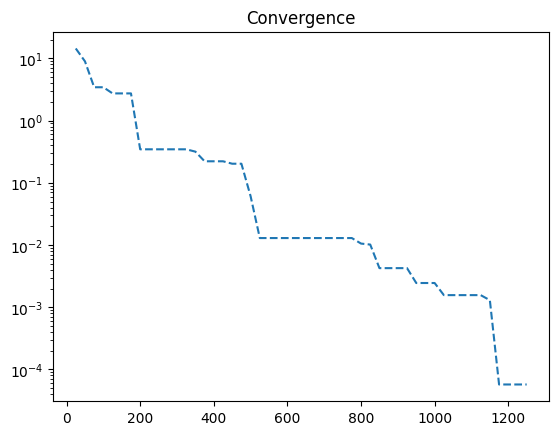
n_evals = np.array([e.evaluator.n_eval for e in res.history])
opt = np.array([e.opt[0].F for e in res.history])

plt.title("Convergence")
plt.plot(n_evals, opt, "--")
plt.yscale("log")
plt.show()

Callback

Another way is to define a Callback object, which stores the information necessary to plot the convergence. Make sure to pass the object to the minimize function to get the notifications each iteration of the algorithm.

from pymoo.algorithms.soo.nonconvex.pso import PSO
from pymoo.problems import get_problem
from pymoo.optimize import minimize
from pymoo.core.callback import Callback

class MyCallback(Callback):

    def __init__(self) -> None:
        super().__init__()
        self.n_evals = []
        self.opt = []

    def notify(self, algorithm):
        self.n_evals.append(algorithm.evaluator.n_eval)
        self.opt.append(algorithm.opt[0].F)


problem = get_problem("ackley")
algorithm = PSO()
callback = MyCallback()

res = minimize(problem,
               algorithm,
               callback=callback,
               termination=('n_gen', 50),
               seed=1)

Now the callback object contains the information of each generation which can be used for plotting.

plt.title("Convergence")
plt.plot(callback.n_evals, callback.opt, "--")
plt.yscale("log")
plt.show()

<< Reference Directions

Decomposition >>