Constraint Handling¶

Info

Note that since version 0.6.0, the problem attribute n_constr has been replaced by n_ieq_constr and n_eq_constr to define either the number of inequality or equality constraints.

Constraint Handling is essential for solving a real-world optimization problem. Different ways have been proposed in the literature to deal with inequality and equality constraints during optimization. A few ways will be described in this tutorial to give users of pymoo a starting point for how to solve optimization problems with constraints.

In this tutorial, we are going to have a look at the following constrained single-objective optimization problem:

\begin{align} \begin{split} \max \;\; & f(x) = x_1^2 + x_2^2 \\[1mm] \text{s.t.} \;\; & g(x) : x_1 + x_2 \geq 1 \\[2mm] & 0 \leq x_1 \leq 2 \\ & 0 \leq x_2 \leq 2 \end{split} \end{align}

[1]:

from pymoo.core.problem import ElementwiseProblem

class ConstrainedProblem(ElementwiseProblem):

    def __init__(self, **kwargs):
        super().__init__(n_var=2, n_obj=1, n_ieq_constr=1, n_eq_constr=0, xl=0, xu=2, **kwargs)

    def _evaluate(self, x, out, *args, **kwargs):
        out["F"] = x[0] ** 2 + x[1] ** 2
        out["G"] = 1.0 - (x[0] + x[1])

For the problem defined above, the inequality constraint ensures that \(1.0 - (x_1 + x_2) \leq 0.0\) or in other words \(x_1 + x_2 \geq 1.0\). The objective functions wants to minimize the sum of both variables squared and thus the contour plot looks as follows:

[2]:

import numpy as np
import matplotlib.pyplot as plt

X1, X2 = np.meshgrid(np.linspace(0, 2, 500), np.linspace(0, 2, 500))

F = X1**2 + X2**2
plt.rc('font', family='serif')

levels = 5 * np.linspace(0, 1, 10)
plt.figure(figsize=(7, 5))
CS = plt.contour(X1, X2, F, levels, colors='black', alpha=0.5)
CS.collections[0].set_label("$f(x)$")

X = np.linspace(0, 1, 500)
plt.plot(X, 1-X, linewidth=2.0, color="green", linestyle='dotted', label="g(x)")

plt.scatter([0.5], [0.5], marker="*", color="red", s=200, label="Optimum (0.5, 0.5)")

plt.xlim(0, 2)
plt.ylim(0, 2)
plt.xlabel("$x_1$")
plt.ylabel("$x_2$")

plt.legend(loc='upper center', bbox_to_anchor=(0.5, 1.12),
          ncol=4, fancybox=True, shadow=False)

plt.tight_layout()
plt.show()

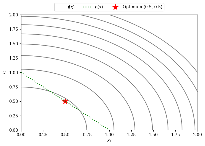
The optimal solution is given by: \(x^{(opt)} = (0.5, 0.5)\) with an objective value \(f(x^{(opt)}) = 0.5\)

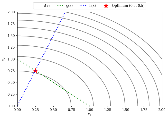
Now let us introduce another constraint, this time an equality constraint.

Note

Next, most algorithms in pymoo will not handle equality constraints efficiently. One reason is the strictness of equality constraints with makes it especially challenging to handle them when solving black-box optimization problems.

\begin{align} \begin{split} \max \;\; & f(x) = x_1^2 + x_2^2 \\[1mm] \text{s.t.} \;\; & g(x) : x_1 + x_2 \geq 1 \\[2mm] \;\; & h(x): 3 x_1 - x_2 = 0 \\[2mm] & 0 \leq x_1 \leq 2 \\ & 0 \leq x_2 \leq 2 \end{split} \end{align}

[3]:

class ConstrainedProblemWithEquality(ElementwiseProblem):

    def __init__(self, **kwargs):
        super().__init__(n_var=2, n_obj=1, n_ieq_constr=1, n_eq_constr=1, xl=0, xu=1, **kwargs)

    def _evaluate(self, x, out, *args, **kwargs):
        out["F"] = x[0] + x[1]
        out["G"] = 1.0 - (x[0] + x[1])
        out["H"] = 3 * x[0] - x[1]

The equality constraint is only satisfied if \(3 \cdot x_1 - x_2 \approx 0\) or in other words \(3\cdot x_1 \approx x_2\).

[4]:

import numpy as np
import matplotlib.pyplot as plt

X1, X2 = np.meshgrid(np.linspace(0, 2, 500), np.linspace(0, 2, 500))

F = X1**2 + X2**2
plt.rc('font', family='serif')

levels = 5 * np.linspace(0, 1, 10)
plt.figure(figsize=(7, 5))
CS = plt.contour(X1, X2, F, levels, colors='black', alpha=0.5)
CS.collections[0].set_label("$f(x)$")

X = np.linspace(0, 1, 500)
plt.plot(X, 1-X, linewidth=2.0, color="green", linestyle='dotted', label="g(x)")
plt.plot(X, 3*X, linewidth=2.0, color="blue", linestyle='dotted', label="h(x)")

plt.scatter([0.25], [0.75], marker="*", color="red", s=200, label="Optimum (0.5, 0.5)")

plt.xlim(0, 2)
plt.ylim(0, 2)
plt.xlabel("$x_1$")
plt.ylabel("$x_2$")

plt.legend(loc='upper center', bbox_to_anchor=(0.5, 1.12),
          ncol=4, fancybox=True, shadow=False)

plt.tight_layout()
plt.show()

The two constrained problems above will be used from now on and solved using different approaches.

Overview

Feasibility First: This is how most algorithms in pymoo handle constraints. Because most of them are based on the sorting of individuals, they simply always prefer feasible solutions over infeasible ones (no matter how much a solution is infeasible). This is a very greedy approach; however, easy to implement across many algorithms in a framework.
Penalty: The optimization problem is redefined by adding a penalty to the objective values. This results in an unconstraint problem that the majority of solvers can handle.
Constraint Violation (CV) As Objective: Another way of considering constraints is treating the constraint violation as an additional objective. This results in a multi-objective problem with one more objective to be solved.
eps-Constraint Handling: Use a dynamic threshold to decide whether a solution is feasible or not. This needs to be implemented by the algorithm.
Repair Operator: Repair a solution to satisfy all (or most) constraints.
Algorithm directly proposed to handled different type of constraints: SRES, ISRES